One Dimensional Equation Of Heat Conduction

ONE DIMENSIONAL EQUATION OF HEAT CONDUCTION

§ "Temperature - gradient".

Consider a homogeneous bar of cross sectional area A. Take the origin O at one end of the bar and the positive x axis along the direction of heat flow. Let PQ be an element of length Ax and u (x, t), u (x + Ax, t) be the temperatures at time t at the ends P and Q respectively.

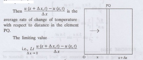
i.e., the potential derivative is the rate of change of temperature w.r.to distance, at p distant x from O. This is called the temperature gradient.

Example 3.4.1: What are the assumptions made while deriving one dimensional heat equation?

Solution: We assume the following experimental laws.

1. Heat flows from higher to lower temperature.

2. The amount of heat required to produce a given temperature change in a body is proportional to the mass of the body and to the temperature change. This constant of proportionality is known mo as the specific heat of the conducting material.

It is known as Fourier’s law of  heat conduction.

Example 3.4.2: State Fourier's law of heat conduction.

The rate at which heat flows across any area is proportional to the area and to the temperature gradient normal to the curve. This constant of proportionality is known as as the thermal conductivity (k y (k) of the material.

It is known as Fourier's law of heat conduction.

Let R₁ be the rate at which heat enters the element PQ of the

bar of cross sectional area A. Then 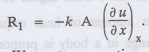 This is mathematical form of Fourier's law. We put a negative sign, as is negative. Heat flows from higher to lower temperature. As x increases, u decreases.

Note: The rate at which heat flows across any area is jointly proportional to the area and to the temperature gradient normal to the area.

Example 3.4.3: Write the p.d.e. of the one dimension heat flow.

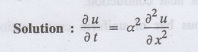
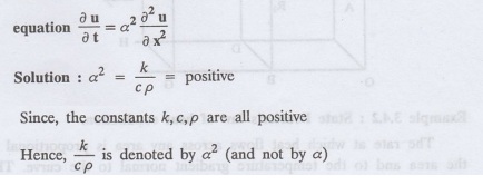
Example 3.4.4 : The p.d.e. of one dimensional heat equation is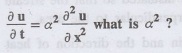 

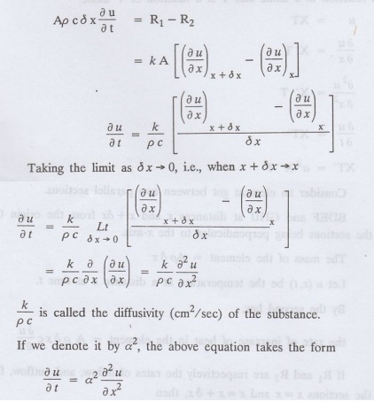
Solution: a² is called the diffusivity of the material of the body through which heat flows. If p be the density, c the specific heat and k thermal conductivity of the material, we have the relation 

Example 3.4.5. Explain why a² (instead of a) is used in the heat equation

 

§ ONE DIMENSIONAL HEAT FLOW

We assume the following experimental laws to get the one dimensional heat flow equation.

1. Heat flows from higher to lower temperature.

2. The amount of heat required to produce a given temperature change in a body is proportional to the mass of the body and to temperature change. This constant of proportionality is known as the specific heat of the conducting material.

3. The rate at which heat flows across any area is proportional to ylnicthe area and to the temperature gradient normal to the curve. This constant of proportionality is known as the thermal conductivity (k) of the material.

It is known as Fourier's law of heat conduction.

Let us consider a homogeneous bar of uniform cross sectional area A.

Assume that the sides of the bar are insulated so that the stream Assume that the lines of he of heat flow are all parallel and perpendicular to the area.

Take an end of the bar as the origin and the direction of heat flow as the positive x-axis.

Let c be the specific heat and k the thermal conductivity of the material.

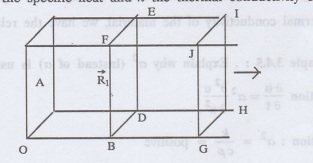
Consider an element got between two parallel sections.

BDEF and GHIJ at distances x and x + dx from the origin O, the sections being perpendicular to the x-axis.

The mass of the element = Αρδχ

Let u (x, t) be the temperature at a distance x at time t.

By the second law,

the rate of increase of heat in the element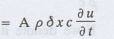 

If R₁ and R₂ are respectively the rates of inflow, and outflow, for the sections x = x and x = x + dx, then

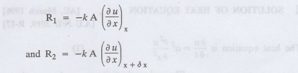
the negative sign being due to the fact that heat flows from higher to lower temperature.

Equating the rate of increase of heat from the two empirical laws,

§ SOLUTION OF HEAT EQUATION

Example 3.4.6: How many boundary conditions are required to solve

Example 3.4.7: State one dimensional heat equation with the initial and boundary conditions.

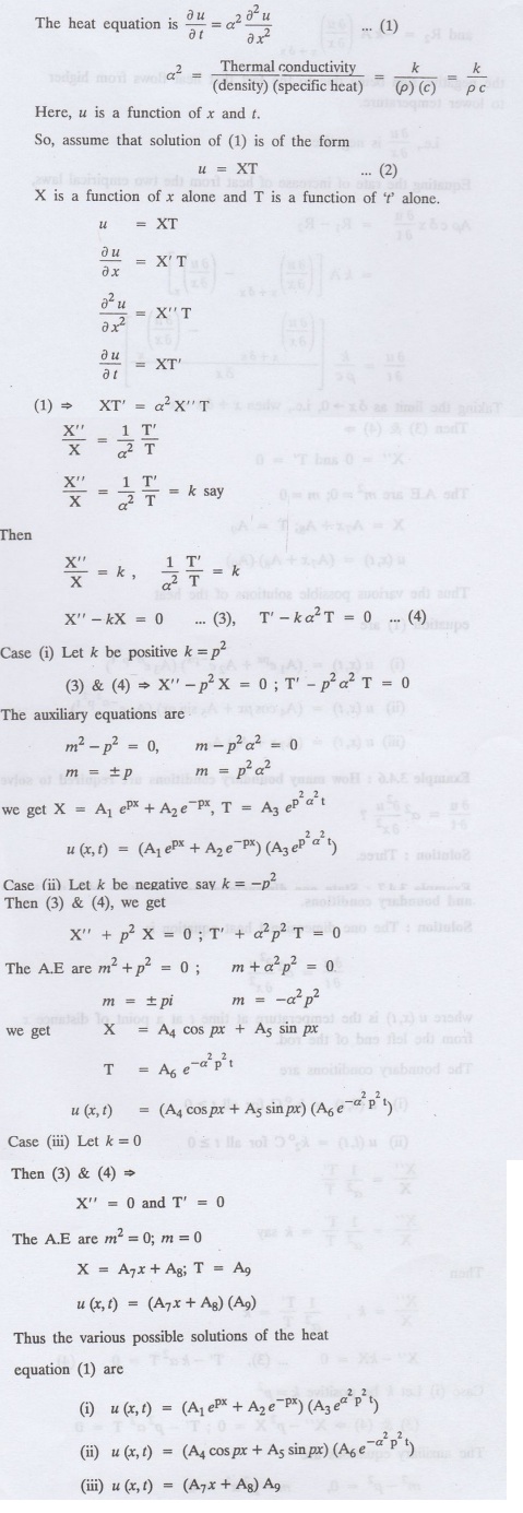
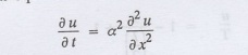
Solution: The one dimensional heat equation is

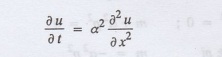
where u (x, t) is the temperature at time t at a point of distance x from the left end of the rod.

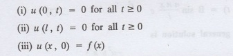
The boundary conditions are

(i) u (0,t) = k₁°C for all t≥ 0

 (ii) u (l,t) = k₂°C for all t≥ 0

 (1 being the length of the one dimensional rod)

The initial condition is

(iii) u (x, 0) = f(x), 0 <x<l 

 

(a) Problems with zero boundary values

 (Temperature or temperature gradients)

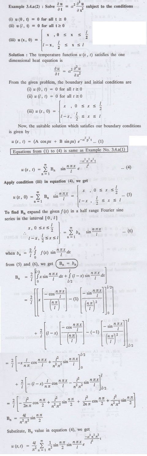
Example 3.4.a(1): A rod of length / with insulated side is initially at a uniform temperature f (x). Its ends are suddenly cooled to 0° C and are kept at the temperature. Find the temperature function u(x, t).

(OR)

Solve the equation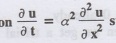subject to the conditions u (0, t)=0,

u (l, t) = 0 and u(x, 0) = f(x).

Solution: The temperature function u (x, t) satisfies the one dimensional heat equation is

From the given problem, we get the following boundary and initial conditions.

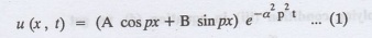
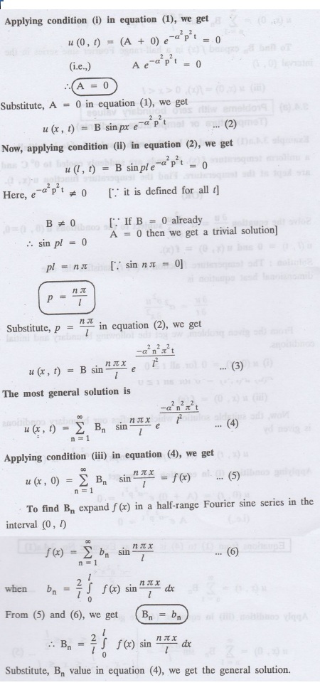
Now, the suitable solution which satisfies our boundary conditions is given by

Applying condition (i) in equation (1), we get

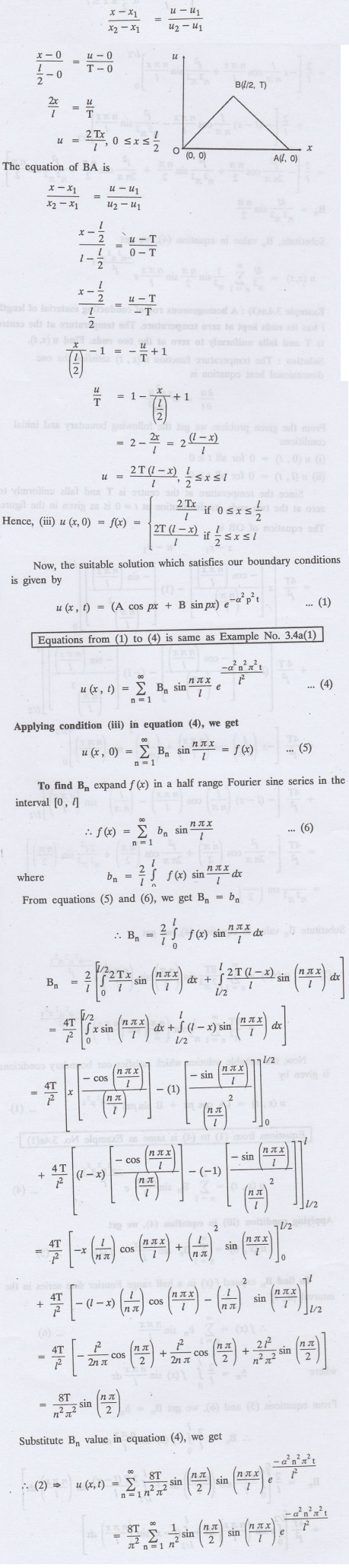
Example 3.4.a(3): A homogeneous rod of conducting material of length I has its ends kept at zero temperature. The temperature at the centre is T and falls uniformly to zero at the two ends. Find u (x, t).

Solution: The temperature function u (x, t) satisfies the one dimensional heat equation

From the given problem we get the following boundary and initial conditions

(i) u (0, t) 0 for all t≥0

(ii) u (1,t) 0 for all t≥0

Since the temperature at the centre is T and falls uniformly to zero at the two ends, its distribution at t = 0 is as given in the figure.